Factor-based Asset Pricing Models
General approach
Factor-based Asset Pricing Models (asset pricing models for short) help imposing the additional structure on parameters  and and  of the analytical model. Restrictions, imposed by an asset pricing model, reduce the number of model parameters that need to be estimated and force “rational” investors to allocate wealth among riskless asset and selected factors only, ignoring the rest of the risky assets. Particular cases of asset pricing models are CAPM and Fama-French 3-Factor Model. of the analytical model. Restrictions, imposed by an asset pricing model, reduce the number of model parameters that need to be estimated and force “rational” investors to allocate wealth among riskless asset and selected factors only, ignoring the rest of the risky assets. Particular cases of asset pricing models are CAPM and Fama-French 3-Factor Model.
Linear Regression Equation
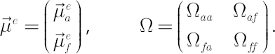
Assume that the financial market consists of  financial instruments, first financial instruments, first  of which we denote as assets, the others of which we denote as assets, the others  we denote as factors1. It is supposed that the dynamics of the market satisfies the conditions of the analytical model with we denote as factors1. It is supposed that the dynamics of the market satisfies the conditions of the analytical model with  excess Mu vector excess Mu vector  and and  covariance matrix covariance matrix  . The given parameters can be decomposed according to . The given parameters can be decomposed according to  assets and assets and  factors: factors:
Let us denote through  vectors of simple rates of return for assets and factors respectively on the interval vectors of simple rates of return for assets and factors respectively on the interval 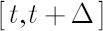 , where , where  is small enough. is small enough.
Dependence of  from from  can be expressed by the linear regression equation can be expressed by the linear regression equation
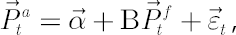
where
 is the is the  vector of mispricing terms (Jensen’s instantaneous alphas); vector of mispricing terms (Jensen’s instantaneous alphas);
 is the is the  matrix of factor sensitivities (Betas); matrix of factor sensitivities (Betas);
 is random vector of residuals with zero average is random vector of residuals with zero average  and such a covariance matrix and such a covariance matrix  that components of vectors and that components of vectors and  are uncorrelated. are uncorrelated.
The elements  of matrix of matrix  are known as residual variances. Their roots are referred to as standard errors of forecast, implied by the regression. are known as residual variances. Their roots are referred to as standard errors of forecast, implied by the regression.
Let us denote sample estimates of and through 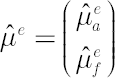 and and 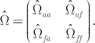
Estimates of parameters  and are found by means of ordinary least-squares using the following formulas: and are found by means of ordinary least-squares using the following formulas:
Model Assumptions
The asset pricing model imposes the following restrictions, which must be satisfied by the above regression equation:
 . .
All mispricing terms in regression equation must be equal to zero.
 is diagonal. is diagonal.
Regression residuals must be uncorrelated.
Practical Implications
If selected asset pricing model holds true, then the main implication for a CRRA investor (an investor with CRRA utility function) is that there is no sense to invest in individual assets. Corresponding optimal portfolio would contain only riskless asset and portfolio factors as its components. Of course, this is true only when selected factors are available for an investment (i.e. they are at least tradable financial instruments).
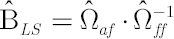
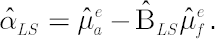
Model-implied Estimates of and
Assuming that the asset pricing model holds true, leads to the modified estimates for and . Model-implied estimates  and and  are given by the following formulas: are given by the following formulas:
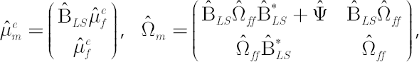
where the matrix  is diagonal and is diagonal and 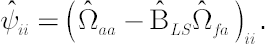
Portfolio Statistics
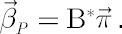
Portfolio Beta
Consider portfolio  . Vector . Vector  of portfolio betas can be found in the following way: of portfolio betas can be found in the following way:
Portfolio Variance
Under the selected set of factors the portfolio variance  admits the following decomposition admits the following decomposition
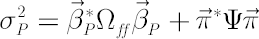
into systematic risk (first item) and diversifiable (nonsystematic) risk (second one).
Other Statistics
Other useful formulae related to asset pricing models include:
 Statistics Statistics
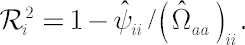
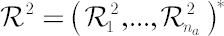 is is  vector, whose elements take values in vector, whose elements take values in  . It is called determination coefficient. The more the value . It is called determination coefficient. The more the value  is closer to unity, the better the selected asset pricing model describes the dynamics of is closer to unity, the better the selected asset pricing model describes the dynamics of  -th asset. Calculation formula: -th asset. Calculation formula:
Student’s  -statistics for vector and matrix -statistics for vector and matrix
-statistics are used in linear regression for testing of hypotheses about regression coefficients beingequal to zero. Formulas for the calculation of -statistics 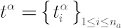 and and 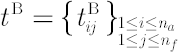 are presented below. are presented below.
Assume that  is the sample size on which the regression coefficients were estimated, and is the sample size on which the regression coefficients were estimated, and  is a number of years contained in sample. Then is a number of years contained in sample. Then
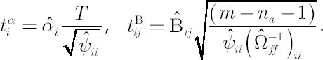
The critical two-sided probabilities for Student’s -distribution with  degrees of freedom are obtained based on the absolute values of the calculated statistics. If degrees of freedom are obtained based on the absolute values of the calculated statistics. If  , then one may use normal distribution instead of -distribution. The values obtained in this way are probabilities of the corresponding regression coefficients being equal to zero. , then one may use normal distribution instead of -distribution. The values obtained in this way are probabilities of the corresponding regression coefficients being equal to zero.
Note. The following rule of thumb can be proposed: if the absolute value of statistics is more than 3, and the number of degrees of freedom is not less than 10, then with high probability (about 99%) the corresponding regression coefficient is significant.
1 Readers shall not confuse the subscript  used in this section with the riskless rate symbol used in this section with the riskless rate symbol  . .
| |
|
 SiteMap\
 Contact Us
 The Theory
\
Details
\
asset-pricing models
\
general approach
The Theory
\
Details
\
asset-pricing models
\
general approach